We’re at an exciting inflection point in the widespread adoption of machine learning (ML), and we believe most customer experiences and applications will be reinvented with generative AI. Generative AI can create new content and ideas, including conversations, stories, images, videos, and music. Like most AI, generative AI is powered by ML models—very large models that are trained on vast amounts of data and commonly referred to as foundation models (FMs). FMs are based on transformers. Transformers are slow and memory-hungry on generating long text sequences due to the sheer size of the models. Large language models (LLMs) used to generate text sequences need immense amounts of computing power and have difficulty accessing the available high bandwidth memory (HBM) and compute capacity. This is because a large portion of the available memory bandwidth is consumed by loading the model’s parameters and by the auto-regressive decoding process.As a result, even with massive amounts of compute power, LLMs are limited by memory I/O and computation limits, preventing them from taking full advantage of the available hardware resources.
Overall, generative inference of LLMs has three main challenges (according to Pope et al. 2022):
- A large memory footprint due to massive model parameters and transient state during decoding. The parameters often exceed the memory of a single accelerator chip. Attention key-value caches also require substantial memory.
- Low parallelizability increases latency, especially with the large memory footprint, requiring substantial data transfers to load parameters and caches into compute cores each step. This results in high total memory bandwidth needs to meet latency targets.
- Quadratic scaling of attention mechanism compute relative to sequence length compounds the latency and computational challenges.
Batching is one of the techniques to address these challenges. Batching refers to the process of sending multiple input sequences together to a LLM and thereby optimizing the performance of the LLM inference. This approach helps improve throughput because model parameters don’t need to be loaded for every input sequence. The parameters can be loaded one time and used to process multiple input sequences. Batching efficiently utilizes the accelerator’s HBM bandwidth, resulting in higher compute utilization, improved throughput, and cost-effective inference.
This post examines techniques to maximize the throughput using batching techniques for parallelized generative inference in LLMs. We discuss different batching methods to reduce memory footprint, increase parallelizability, and mitigate the quadratic scaling of attention to boost throughput. The goal is to fully use hardware like HBM and accelerators to overcome bottlenecks in memory, I/O, and computation. Then we highlight how Amazon SageMaker large model inference (LMI) deep learning containers (DLCs) can help with these techniques. Finally, we present a comparative analysis of throughput improvements with each batching strategy on SageMaker using LMI DLCs to improve throughput for models like Llama v2. You can find an accompanying example notebook in the SageMaker examples GitHub repository.
Inferencing for large language models (LLMs)
Autoregressive decoding is the process by which language models like GPT generate text output one token at a time. It involves recursively feeding generated tokens back into the model as part of the input sequence in order to predict subsequent tokens. The steps are as follows:
- The model receives the previous tokens in the sequence as input. For the first step, this is the starting prompt provided by the user.
- The model predicts a distribution over the vocabulary for the next token.
- The token with the highest predicted probability is selected and appended to the output sequence. Steps 2 and 3 are part of the decoding As of this writing, the most prominent decoding methods are greedy search, beam search, contrastive search, and sampling.
- This new token is added to the input sequence for the next decoding step.
- The model iterates through these steps, generating one new token per step, until an end-of-sequence marker is produced or the desired output length is reached.
Model serving for LLMs
Model serving for LLMs refers to the process of receiving input requests for text generation, making inferences, and returning the results to the requesting applications. The following are key concepts involved in model serving:
- Clients generate multiple inference requests, with each request consisting of sequence of tokens or input prompts
- Requests are received by the inference server (for example, DJLServing, TorchServe, Triton, or Hugging Face TGI)
- The inference server batches the inference requests and schedules the batch to the execution engine that includes model partitioning libraries (such as Transformers-NeuronX, DeepSpeed, Accelerate, or FasterTransformer) for running the forward pass (predicting the output token sequence) on the generative language model
- The execution engine generates response tokens and sends the response back to the inference server
- The inference server replies to the clients with the generated results

There are challenges with request-level scheduling when the inference server interacts with the execution engine at the request level, such as each request using a Python process, which requires a separate copy of model, which is memory restrictive. For example, as shown in the following figure, you can only accommodate to load a single copy of a model of size 80 GB on a machine learning (ML) instance with 96 GB of total accelerator device memory. You will need to load an additional copy of the entire model if you want to serve additional requests concurrently. This is not memory and cost efficient.

Now that we understand challenges posed by request-level scheduling, let’s look at different batching techniques that can help optimize throughput.
Batching techniques
In this section, we explain different batching techniques and show how to implement them using a SageMaker LMI container.

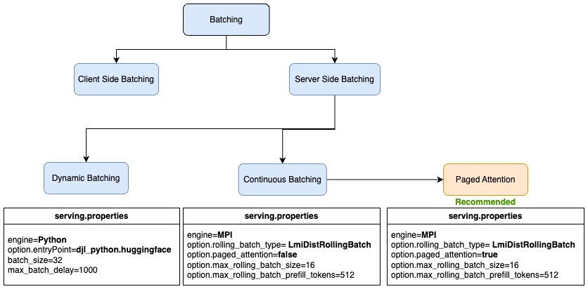
There are two main types of batching for inference requests:
- Client-side (static) – Typically, when a client sends a request to a server, the server will process each request sequentially by default, which is not optimal for throughput. To optimize the throughput, the client batches the inference requests in the single payload and the server implements the preprocessing logic to break down the batch into multiple requests and runs the inference for each request separately. In this option, the client needs to change the code for batching and the solution is tightly coupled with the batch size.
- Server-side (dynamic) – Another technique for batching is to use the inference to help achieve the batching on server side. As independent inference requests arrive at the server, the inference server can dynamically group them into larger batches on the server side. The inference server can manage the batching to meet a specified latency target, maximizing throughput while staying within the desired latency range. The inference server handles this automatically, so no client-side code changes are needed. The server-side batching includes different techniques to optimize the throughput further for generative language models based on the auto-regressive decoding. These batching techniques include dynamic batching, continuous batching, and PagedAttention (vLLM) batching.
Dynamic batching
Dynamic batching refers to combining the input requests and sending them together as a batch for inference. Dynamic batching is a generic server-side batching technique that works for all tasks, including computer vision (CV), natural language processing (NLP), and more.
In an LMI container, you can configure the batching of requests based on the following settings in serving.properties:
- batch_size – Refers to the size of the batch
- max_batch_delay – Refers to the maximum delay for batch aggregation
If either of these thresholds are met (meeting the maximum batch size or completion of the waiting period), then a new batch is prepared and pushed to the model for inferencing. The following diagram shows the dynamic batching of requests with different input sequence lengths being processed together by the model.

You can implement dynamic batching on SageMaker by configuring the LMI container’s serving.properties as follows:
Although dynamic batching can provide up to a four-times increase in throughput compared to no batching, we observe that GPU utilization is not optimal in this case because the system can’t accept another batch until all requests have completed processing.
Continuous batching
Continuous batching is an optimization specific for text generation. It improves throughput and doesn’t sacrifice the time to first byte latency. Continuous batching (also known as iterative or rolling batching) addresses the challenge of idle GPU time and builds on top of the dynamic batching approach further by continuously pushing newer requests in the batch. The following diagram shows continuous batching of requests. When requests 2 and 3 finish processing, another set of requests is scheduled.

The following interactive diagram dives deeper into how continuous batching works.

(Courtesy: https://github.com/InternLM/lmdeploy)
You can use a powerful technique to make LLMs and text generation efficient: caching some of the attention matrices. This means that the first pass of a prompt is different from the subsequent forward passes. For the first pass, you have to compute the entire attention matrix, whereas the follow-ups only require you to compute the new token attention. The first pass is called prefill throughout this code base, whereas the follow-ups are called decode. Because prefill is much more expensive than decode, we don’t want to do it all the time, but a currently running query is probably doing decode. If we want to use continuous batching as explained previously, we need to run prefill at some point in order to create the attention matrix required to be able to join the decode group.
This technique may allow up to a 20-times increase in throughput compared to no batching by effectively utilizing the idle GPUs.
You can fine-tune the following parameters in serving.properties of the LMI container for using continuous batching:
- engine – The runtime engine of the code. Values include
Python,DeepSpeed,FasterTransformer, andMPI. UseMPIto enable continuous batching. - rolling_batch – Enables iteration-level batching using one of the supported strategies. Values include
auto,scheduler, andlmi-dist. We uselmi-distfor turning on continuous batching for Llama 2. - max_rolling_batch_size – Limits the number of concurrent requests in the continuous batch. Defaults to 32.
- max_rolling_batch_prefill_tokens – Limits the number of tokens for caching. This needs to be tuned based on batch size and input sequence length to avoid GPU out of memory. It’s only supported for when
rolling_batch=lmi-dist. Our recommendation is to set the value based on the number of concurrent requests x the memory required to store input tokens and output tokens per request.
The following is sample code for serving.properties for configuring continuous batching:
PagedAttention batching
In the autoregressive decoding process, all the input tokens to the LLM produce their attention key and value tensors, and these tensors are kept in GPU memory to generate next tokens. These cached key and value tensors are often referred to as the KV cache or attention cache. As per the paper vLLM: Easy, Fast, and Cheap LLM Serving with PagedAttention, the KV cache takes up to 1.7 GB for a single sequence in Llama 13B. It is also dynamic. Its size depends on the sequence length, which is highly variable and unpredictable. As a result, efficiently managing the KV cache presents a significant challenge. The paper found that existing systems waste 60–80% of memory due to fragmentation and over-reservation.
PagedAttention is a new optimization algorithm developed by UC Berkeley that improves the continuous batching process by allowing the attention cache (KV cache) to be non-contiguous by allocating memory in fixed-size pages or blocks. This is inspired by virtual memory and paging concepts used by operating systems.
As per the vLLM paper, the attention cache of each sequence of tokens is partitioned into blocks and mapped to physical blocks through a block table. During the computation of attention, a PagedAttention kernel can use the block table to efficiently fetch the blocks from physical memory. This results in a significant reduction of memory waste and allows for larger batch size, increased GPU utilization, and higher throughput. The following figure illustrates partitioning the attention cache into non-contiguous pages.

The following diagram shows an inference example with PagedAttention. The key steps are:
- The inference request is received with an input prompt.
- In the prefill phase, attention is computed and key-values are stored in non-contiguous physical memory and mapped to logical key-value blocks. This mapping is stored in a block table.
- The input prompt is run through the model (a forward pass) to generate the first response token. During the response token generation, the attention cache from the prefill phase is used.
- During subsequent token generation, if the current physical block is full, additional memory is allocated in a non-contiguous fashion, allowing just-in-time allocation.

PagedAttention helps in near-optimal memory usage and reduction of memory waste. This allows for more requests to be batched together, resulting in a significant increase in throughput of inferencing.
The following code is a sample serving.properties for configuring PagedAttention batching in an LMI container on SageMaker:
When to use which batching technique
The following figure summarizes the server-side batching techniques along with the sample serving.properties in LMI on SageMaker.
The following table summarizes the different batching techniques and their use cases.
| PagedAttention Batching | Continuous Batching | Dynamic Batching | Client-side Batching | No Batch | |
| How it works | Always merge new requests at the token level along with paged blocks and do batch inference. | Always merge new request at the token level and do batch inference. | Merge the new request at the request level; can delay for a few milliseconds to form a batch. | Client is responsible for batching multiple inference requests in the same payload before sending it to the inference server. | When a request arrives, run the inference immediately. |
| When it works the best | This is the recommended approach for the supported decoder-only models. It’s suitable for throughput-optimized workloads. It’s applicable to only text-generation models. | Concurrent requests coming at different times with the same decoding strategy. It’s suitable for throughput-optimized workloads. It’s applicable to only text-generation models. | Concurrent requests coming at different times with the same decoding strategy. It’s suitable for response time-sensitive workloads needing higher throughput. It’s applicable to CV, NLP, and other types of models. | It’s suitable for offline inference use cases that don’t have latency constraints for maximizing the throughput. | Infrequent inference requests or inference requests with different decoding strategies. It’s suitable for workloads with strict response time latency needs. |
Throughput comparison of different batching techniques for a large generative model on SageMaker
We performed performance benchmarking on a Llama v2 7B model on SageMaker using an LMI container and the different batching techniques discussed in this post with concurrent incoming requests of 50 and a total number of requests of 5,000.
We used three different input prompts of variable lengths for the performance test. In continuous and PagedAttention batching, the output tokens lengths were set to 64, 128, and 256 for the three input prompts, respectively. For dynamic batching, we used a consistent output token length of 128 tokens. We deployed SageMaker endpoints for the test with an instance type of ml.g5.24xlarge. The following table contains the results of the performance benchmarking tests.
| Model | Batching Strategy | Requests per Second on ml.g5.24xlarge |
| LLaMA2-7b | Dynamic Batching | 3.24 |
| LLaMA2-7b | Continuous Batching | 6.92 |
| LLaMA2-7b | PagedAttention Batching | 7.41 |
We see an increase of approximately 2.3 times in throughput by using PagedAttention batching in comparison to dynamic batching for the Llama2-7B model on SageMaker using an LMI container.
Conclusion
In this post, we explained different batching techniques for LLMs inferencing and how it helps increase throughput. We showed how memory optimization techniques can increase the hardware efficiency by using continuous and PagedAttention batching and provide higher throughput values than dynamic batching. We saw an increase of approximately 2.3 times in throughput by using PagedAttention batching in comparison to dynamic batching for a Llama2-7B model on SageMaker using an LMI container. You can find the notebook used for testing the different batching techniques on GitHub.
About the authors
 Gagan Singh is a Senior Technical Account Manager at AWS, where he partners with digital native startups to pave their path to heightened business success. With a niche in propelling Machine Learning initiatives, he leverages Amazon SageMaker, particularly emphasizing on Deep Learning and Generative AI solutions. In his free time, Gagan finds solace in trekking on the trails of the Himalayas and immersing himself in diverse music genres.
 Dhawal Patel is a Principal Machine Learning Architect at AWS. He has worked with organizations ranging from large enterprises to mid-sized startups on problems related to distributed computing, and Artificial Intelligence. He focuses on Deep learning including NLP and Computer Vision domains. He helps customers achieve high performance model inference on SageMaker.
 Venugopal Pai is a Solutions Architect at AWS. He lives in Bengaluru, India, and helps digital native customers scale and optimize their applications on AWS.
- SEO Powered Content & PR Distribution. Get Amplified Today.
- PlatoData.Network Vertical Generative Ai. Empower Yourself. Access Here.
- PlatoAiStream. Web3 Intelligence. Knowledge Amplified. Access Here.
- PlatoESG. Carbon, CleanTech, Energy, Environment, Solar, Waste Management. Access Here.
- PlatoHealth. Biotech and Clinical Trials Intelligence. Access Here.
- Source: https://aws.amazon.com/blogs/machine-learning/improve-throughput-performance-of-llama-2-models-using-amazon-sagemaker/