Machine learning (ML) is becoming increasingly complex as customers try to solve more and more challenging problems. This complexity often leads to the need for distributed ML, where multiple machines are used to train a single model. Although this enables parallelization of tasks across multiple nodes, leading to accelerated training times, enhanced scalability, and improved performance, there are significant challenges in effectively using distributed hardware. Data scientists have to address challenges like data partitioning, load balancing, fault tolerance, and scalability. ML engineers must handle parallelization, scheduling, faults, and retries manually, requiring complex infrastructure code.
In this post, we discuss the benefits of using Ray and Amazon SageMaker for distributed ML, and provide a step-by-step guide on how to use these frameworks to build and deploy a scalable ML workflow.
Ray, an open-source distributed computing framework, provides a flexible framework for distributed training and serving of ML models. It abstracts away low-level distributed system details through simple, scalable libraries for common ML tasks such as data preprocessing, distributed training, hyperparameter tuning, reinforcement learning, and model serving.
SageMaker is a fully managed service for building, training, and deploying ML models. Ray seamlessly integrates with SageMaker features to build and deploy complex ML workloads that are both efficient and reliable. The combination of Ray and SageMaker provides end-to-end capabilities for scalable ML workflows, and has the following highlighted features:
- Distributed actors and parallelism constructs in Ray simplify developing distributed applications.
- Ray AI Runtime (AIR) reduces friction of going from development to production. With Ray and AIR, the same Python code can scale seamlessly from a laptop to a large cluster.
- The managed infrastructure of SageMaker and features like processing jobs, training jobs, and hyperparameter tuning jobs can use Ray libraries underneath for distributed computing.
- Amazon SageMaker Experiments allows rapidly iterating and keeping track of trials.
- Amazon SageMaker Feature Store provides a scalable repository for storing, retrieving, and sharing ML features for model training.
- Trained models can be stored, versioned, and tracked in Amazon SageMaker Model Registry for governance and management.
- Amazon SageMaker Pipelines allows orchestrating the end-to-end ML lifecycle from data preparation and training to model deployment as automated workflows.
Solution overview
This post focuses on the benefits of using Ray and SageMaker together. We set up an end-to-end Ray-based ML workflow, orchestrated using SageMaker Pipelines. The workflow includes parallel ingestion of data into the feature store using Ray actors, data preprocessing with Ray Data, training models and hyperparameter tuning at scale using Ray Train and hyperparameter optimization (HPO) tuning jobs, and finally model evaluation and registering the model into a model registry.
For our data, we use a synthetic housing dataset that consists of eight features (YEAR_BUILT, SQUARE_FEET, NUM_BEDROOM, NUM_BATHROOMS, LOT_ACRES, GARAGE_SPACES, FRONT_PORCH, and DECK) and our model will predict the PRICE of the house.
Each stage in the ML workflow is broken into discrete steps, with its own script that takes input and output parameters. In the next section, we highlight key code snippets from each step. The full code can be found on the aws-samples-for-ray GitHub repository.
Prerequisites
To use the SageMaker Python SDK and run the code associated with this post, you need the following prerequisites:
Ingest data into SageMaker Feature Store
The first step in the ML workflow is to read the source data file from Amazon Simple Storage Service (Amazon S3) in CSV format and ingest it into SageMaker Feature Store. SageMaker Feature Store is a purpose-built repository that makes it easy for teams to create, share, and manage ML features. It simplifies feature discovery, reuse, and sharing, leading to faster development, increased collaboration within customer teams, and reduced costs.
Ingesting features into the feature store contains the following steps:
- Define a feature group and create the feature group in the feature store.
- Prepare the source data for the feature store by adding an event time and record ID for each row of data.
- Ingest the prepared data into the feature group by using the Boto3 SDK.
In this section, we only highlight Step 3, because this is the part that involves parallel processing of the ingestion task using Ray. You can review the full code for this process in the GitHub repo.
The ingest_features method is defined inside a class called Featurestore. Note that the Featurestore class is decorated with @ray.remote. This indicates that an instance of this class is a Ray actor, a stateful and concurrent computational unit within Ray. It’s a programming model that allows you to create distributed objects that maintain an internal state and can be accessed concurrently by multiple tasks running on different nodes in a Ray cluster. Actors provide a way to manage and encapsulate the mutable state, making them valuable for building complex, stateful applications in a distributed setting. You can specify resource requirements in actors too. In this case, each instance of the FeatureStore class will require 0.5 CPUs. See the following code:
@ray.remote(num_cpus=0.5)
class Featurestore: def ingest_features(self,feature_group_name, df, region): """ Ingest features to Feature Store Group Args: feature_group_name (str): Feature Group Name data_path (str): Path to the train/validation/test data in CSV format. """ ...
You can interact with the actor by calling the remote operator. In the following code, the desired number of actors is passed in as an input argument to the script. The data is then partitioned based on the number of actors and passed to the remote parallel processes to be ingested into the feature store. You can call get on the object ref to block the execution of the current task until the remote computation is complete and the result is available. When the result is available, ray.get will return the result, and the execution of the current task will continue.
import modin.pandas as pd
import ray df = pd.read_csv(s3_path)
data = prepare_df_for_feature_store(df)
# Split into partitions
partitions = [ray.put(part) for part in np.array_split(data, num_actors)]
# Start actors and assign partitions in a loop
actors = [Featurestore.remote() for _ in range(args.num_actors)]
results = [] for actor, partition in zip(actors, input_partitions): results.append(actor.ingest_features.remote( args.feature_group_name, partition, args.region ) ) ray.get(results)
Prepare data for training, validation, and testing
In this step, we use Ray Dataset to efficiently split, transform, and scale our dataset in preparation for machine learning. Ray Dataset provides a standard way to load distributed data into Ray, supporting various storage systems and file formats. It has APIs for common ML data preprocessing operations like parallel transformations, shuffling, grouping, and aggregations. Ray Dataset also handles operations needing stateful setup and GPU acceleration. It integrates smoothly with other data processing libraries like Spark, Pandas, NumPy, and more, as well as ML frameworks like TensorFlow and PyTorch. This allows building end-to-end data pipelines and ML workflows on top of Ray. The goal is to make distributed data processing and ML easier for practitioners and researchers.
Let’s look at sections of the scripts that perform this data preprocessing. We start by loading the data from the feature store:
def load_dataset(feature_group_name, region): """ Loads the data as a ray dataset from the offline featurestore S3 location Args: feature_group_name (str): name of the feature group Returns: ds (ray.data.dataset): Ray dataset the contains the requested dat from the feature store """ session = sagemaker.Session(boto3.Session(region_name=region)) fs_group = FeatureGroup( name=feature_group_name, sagemaker_session=session ) fs_data_loc = fs_group.describe().get("OfflineStoreConfig").get("S3StorageConfig").get("ResolvedOutputS3Uri") # Drop columns added by the feature store # Since these are not related to the ML problem at hand cols_to_drop = ["record_id", "event_time","write_time", "api_invocation_time", "is_deleted", "year", "month", "day", "hour"] ds = ray.data.read_parquet(fs_data_loc) ds = ds.drop_columns(cols_to_drop) print(f"{fs_data_loc} count is {ds.count()}") return ds
We then split and scale data using the higher-level abstractions available from the ray.data library:
def split_dataset(dataset, train_size, val_size, test_size, random_state=None): """ Split dataset into train, validation and test samples Args: dataset (ray.data.Dataset): input data train_size (float): ratio of data to use as training dataset val_size (float): ratio of data to use as validation dataset test_size (float): ratio of data to use as test dataset random_state (int): Pass an int for reproducible output across multiple function calls. Returns: train_set (ray.data.Dataset): train dataset val_set (ray.data.Dataset): validation dataset test_set (ray.data.Dataset): test dataset """ # Shuffle this dataset with a fixed random seed. shuffled_ds = dataset.random_shuffle(seed=random_state) # Split the data into train, validation and test datasets train_set, val_set, test_set = shuffled_ds.split_proportionately([train_size, val_size]) return train_set, val_set, test_set def scale_dataset(train_set, val_set, test_set, target_col): """ Fit StandardScaler to train_set and apply it to val_set and test_set Args: train_set (ray.data.Dataset): train dataset val_set (ray.data.Dataset): validation dataset test_set (ray.data.Dataset): test dataset target_col (str): target col Returns: train_transformed (ray.data.Dataset): train data scaled val_transformed (ray.data.Dataset): val data scaled test_transformed (ray.data.Dataset): test data scaled """ tranform_cols = dataset.columns() # Remove the target columns from being scaled tranform_cols.remove(target_col) # set up a standard scaler standard_scaler = StandardScaler(tranform_cols) # fit scaler to training dataset print("Fitting scaling to training data and transforming dataset...") train_set_transformed = standard_scaler.fit_transform(train_set) # apply scaler to validation and test datasets print("Transforming validation and test datasets...") val_set_transformed = standard_scaler.transform(val_set) test_set_transformed = standard_scaler.transform(test_set) return train_set_transformed, val_set_transformed, test_set_transformed
The processed train, validation, and test datasets are stored in Amazon S3 and will be passed as the input parameters to subsequent steps.
Perform model training and hyperparameter optimization
With our data preprocessed and ready for modeling, it’s time to train some ML models and fine-tune their hyperparameters to maximize predictive performance. We use XGBoost-Ray, a distributed backend for XGBoost built on Ray that enables training XGBoost models on large datasets by using multiple nodes and GPUs. It provides simple drop-in replacements for XGBoost’s train and predict APIs while handling the complexities of distributed data management and training under the hood.
To enable distribution of the training over multiple nodes, we utilize a helper class named RayHelper. As shown in the following code, we use the resource configuration of the training job and choose the first host as the head node:
class RayHelper(): def __init__(self, ray_port:str="9339", redis_pass:str="redis_password"): .... self.resource_config = self.get_resource_config() self.head_host = self.resource_config["hosts"][0] self.n_hosts = len(self.resource_config["hosts"])We can use the host information to decide how to initialize Ray on each of the training job instances:
def start_ray(self): head_ip = self._get_ip_from_host() # If the current host is the host choosen as the head node # run `ray start` with specifying the --head flag making this is the head node if self.resource_config["current_host"] == self.head_host: output = subprocess.run(['ray', 'start', '--head', '-vvv', '--port', self.ray_port, '--redis-password', self.redis_pass, '--include-dashboard', 'false'], stdout=subprocess.PIPE) print(output.stdout.decode("utf-8")) ray.init(address="auto", include_dashboard=False) self._wait_for_workers() print("All workers present and accounted for") print(ray.cluster_resources()) else: # If the current host is not the head node, # run `ray start` with specifying ip address as the head_host as the head node time.sleep(10) output = subprocess.run(['ray', 'start', f"--address={head_ip}:{self.ray_port}", '--redis-password', self.redis_pass, "--block"], stdout=subprocess.PIPE) print(output.stdout.decode("utf-8")) sys.exit(0)
When a training job is started, a Ray cluster can be initialized by calling the start_ray() method on an instance of RayHelper:
if __name__ == '__main__': ray_helper = RayHelper() ray_helper.start_ray() args = read_parameters() sess = sagemaker.Session(boto3.Session(region_name=args.region))
We then use the XGBoost trainer from XGBoost-Ray for training:
def train_xgboost(ds_train, ds_val, params, num_workers, target_col = "price") -> Result: """ Creates a XGBoost trainer, train it, and return the result. Args: ds_train (ray.data.dataset): Training dataset ds_val (ray.data.dataset): Validation dataset params (dict): Hyperparameters num_workers (int): number of workers to distribute the training across target_col (str): target column Returns: result (ray.air.result.Result): Result of the training job """ train_set = RayDMatrix(ds_train, 'PRICE') val_set = RayDMatrix(ds_val, 'PRICE') evals_result = {} trainer = train( params=params, dtrain=train_set, evals_result=evals_result, evals=[(val_set, "validation")], verbose_eval=False, num_boost_round=100, ray_params=RayParams(num_actors=num_workers, cpus_per_actor=1), ) output_path=os.path.join(args.model_dir, 'model.xgb') trainer.save_model(output_path) valMAE = evals_result["validation"]["mae"][-1] valRMSE = evals_result["validation"]["rmse"][-1] print('[3] #011validation-mae:{}'.format(valMAE)) print('[4] #011validation-rmse:{}'.format(valRMSE)) local_testing = False try: load_run(sagemaker_session=sess) except: local_testing = True if not local_testing: # Track experiment if using SageMaker Training with load_run(sagemaker_session=sess) as run: run.log_metric('validation-mae', valMAE) run.log_metric('validation-rmse', valRMSE)
Note that while instantiating the trainer, we pass RayParams, which takes the number actors and number of CPUs per actors. XGBoost-Ray uses this information to distribute the training across all the nodes attached to the Ray cluster.
We now create a XGBoost estimator object based on the SageMaker Python SDK and use that for the HPO job.
Orchestrate the preceding steps using SageMaker Pipelines
To build an end-to-end scalable and reusable ML workflow, we need to use a CI/CD tool to orchestrate the preceding steps into a pipeline. SageMaker Pipelines has direct integration with SageMaker, the SageMaker Python SDK, and SageMaker Studio. This integration allows you to create ML workflows with an easy-to-use Python SDK, and then visualize and manage your workflow using SageMaker Studio. You can also track the history of your data within the pipeline execution and designate steps for caching.
SageMaker Pipelines creates a Directed Acyclic Graph (DAG) that includes steps needed to build an ML workflow. Each pipeline is a series of interconnected steps orchestrated by data dependencies between steps, and can be parameterized, allowing you to provide input variables as parameters for each run of the pipeline. SageMaker Pipelines has four types of pipeline parameters: ParameterString, ParameterInteger, ParameterFloat, and ParameterBoolean. In this section, we parameterize some of the input variables and set up the step caching configuration:
processing_instance_count = ParameterInteger( name='ProcessingInstanceCount', default_value=1
)
feature_group_name = ParameterString( name='FeatureGroupName', default_value='fs-ray-synthetic-housing-data'
)
bucket_prefix = ParameterString( name='Bucket_Prefix', default_value='aws-ray-mlops-workshop/feature-store'
)
rmse_threshold = ParameterFloat(name="RMSEThreshold", default_value=15000.0) train_size = ParameterString( name='TrainSize', default_value="0.6"
)
val_size = ParameterString( name='ValidationSize', default_value="0.2"
)
test_size = ParameterString( name='TestSize', default_value="0.2"
) cache_config = CacheConfig(enable_caching=True, expire_after="PT12H")
We define two processing steps: one for SageMaker Feature Store ingestion, the other for data preparation. This should look very similar to the previous steps described earlier. The only new line of code is the ProcessingStep after the steps’ definition, which allows us to take the processing job configuration and include it as a pipeline step. We further specify the dependency of the data preparation step on the SageMaker Feature Store ingestion step. See the following code:
feature_store_ingestion_step = ProcessingStep( name='FeatureStoreIngestion', step_args=fs_processor_args, cache_config=cache_config
) preprocess_dataset_step = ProcessingStep( name='PreprocessData', step_args=processor_args, cache_config=cache_config
)
preprocess_dataset_step.add_depends_on([feature_store_ingestion_step])
Similarly, to build a model training and tuning step, we need to add a definition of TuningStep after the model training step’s code to allow us to run SageMaker hyperparameter tuning as a step in the pipeline:
tuning_step = TuningStep( name="HPTuning", tuner=tuner, inputs={ "train": TrainingInput( s3_data=preprocess_dataset_step.properties.ProcessingOutputConfig.Outputs[ "train" ].S3Output.S3Uri, content_type="text/csv" ), "validation": TrainingInput( s3_data=preprocess_dataset_step.properties.ProcessingOutputConfig.Outputs[ "validation" ].S3Output.S3Uri, content_type="text/csv" ) }, cache_config=cache_config,
)
tuning_step.add_depends_on([preprocess_dataset_step])
After the tuning step, we choose to register the best model into SageMaker Model Registry. To control the model quality, we implement a minimum quality gate that compares the best model’s objective metric (RMSE) against a threshold defined as the pipeline’s input parameter rmse_threshold. To do this evaluation, we create another processing step to run an evaluation script. The model evaluation result will be stored as a property file. Property files are particularly useful when analyzing the results of a processing step to decide how other steps should be run. See the following code:
# Specify where we'll store the model evaluation results so that other steps can access those results
evaluation_report = PropertyFile( name='EvaluationReport', output_name='evaluation', path='evaluation.json',
) # A ProcessingStep is used to evaluate the performance of a selected model from the HPO step. # In this case, the top performing model is evaluated. evaluation_step = ProcessingStep( name='EvaluateModel', processor=evaluation_processor, inputs=[ ProcessingInput( source=tuning_step.get_top_model_s3_uri( top_k=0, s3_bucket=bucket, prefix=s3_prefix ), destination='/opt/ml/processing/model', ), ProcessingInput( source=preprocess_dataset_step.properties.ProcessingOutputConfig.Outputs['test'].S3Output.S3Uri, destination='/opt/ml/processing/test', ), ], outputs=[ ProcessingOutput( output_name='evaluation', source='/opt/ml/processing/evaluation' ), ], code='./pipeline_scripts/evaluate/script.py', property_files=[evaluation_report],
)
We define a ModelStep to register the best model into SageMaker Model Registry in our pipeline. In case the best model doesn’t pass our predetermined quality check, we additionally specify a FailStep to output an error message:
register_step = ModelStep( name='RegisterTrainedModel', step_args=model_registry_args
) metrics_fail_step = FailStep( name="RMSEFail", error_message=Join(on=" ", values=["Execution failed due to RMSE >", rmse_threshold]),
)
Next, we use a ConditionStep to evaluate whether the model registration step or failure step should be taken next in the pipeline. In our case, the best model will be registered if its RMSE score is lower than the threshold.
# Condition step for evaluating model quality and branching execution
cond_lte = ConditionLessThanOrEqualTo( left=JsonGet( step_name=evaluation_step.name, property_file=evaluation_report, json_path='regression_metrics.rmse.value', ), right=rmse_threshold,
)
condition_step = ConditionStep( name='CheckEvaluation', conditions=[cond_lte], if_steps=[register_step], else_steps=[metrics_fail_step],
)
Finally, we orchestrate all the defined steps into a pipeline:
pipeline_name = 'synthetic-housing-training-sm-pipeline-ray'
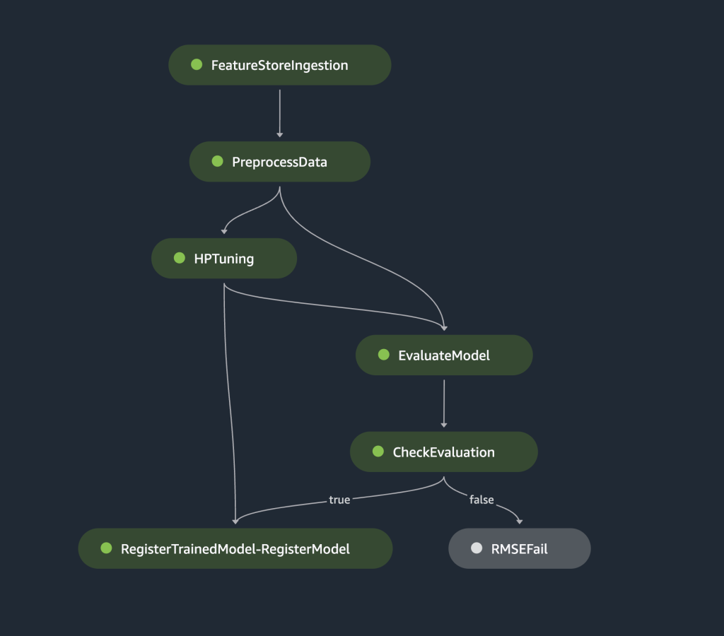
step_list = [ feature_store_ingestion_step, preprocess_dataset_step, tuning_step, evaluation_step, condition_step ] training_pipeline = Pipeline( name=pipeline_name, parameters=[ processing_instance_count, feature_group_name, train_size, val_size, test_size, bucket_prefix, rmse_threshold ], steps=step_list
) # Note: If an existing pipeline has the same name it will be overwritten.
training_pipeline.upsert(role_arn=role_arn)
The preceding pipeline can be visualized and executed directly in SageMaker Studio, or be executed by calling execution = training_pipeline.start(). The following figure illustrates the pipeline flow.
Additionally, we can review the lineage of artifacts generated by the pipeline execution.
from sagemaker.lineage.visualizer import LineageTableVisualizer viz = LineageTableVisualizer(sagemaker.session.Session())
for execution_step in reversed(execution.list_steps()): print(execution_step) display(viz.show(pipeline_execution_step=execution_step)) time.sleep(5)
Deploy the model
After the best model is registered in SageMaker Model Registry via a pipeline run, we deploy the model to a real-time endpoint by using the fully managed model deployment capabilities of SageMaker. SageMaker has other model deployment options to meet the needs of different use cases. For details, refer to Deploy models for inference when choosing the right option for your use case. First, let’s get the model registered in SageMaker Model Registry:
xgb_regressor_model = ModelPackage( role_arn, model_package_arn=model_package_arn, name=model_name
)
The model’s current status is PendingApproval. We need to set its status to Approved prior to deployment:
sagemaker_client.update_model_package( ModelPackageArn=xgb_regressor_model.model_package_arn, ModelApprovalStatus='Approved'
) xgb_regressor_model.deploy( initial_instance_count=1, instance_type='ml.m5.xlarge', endpoint_name=endpoint_name
)
Clean up
After you are done experimenting, remember to clean up the resources to avoid unnecessary charges. To clean up, delete the real-time endpoint, model group, pipeline, and feature group by calling the APIs DeleteEndpoint, DeleteModelPackageGroup, DeletePipeline, and DeleteFeatureGroup, respectively, and shut down all SageMaker Studio notebook instances.
Conclusion
This post demonstrated a step-by-step walkthrough on how to use SageMaker Pipelines to orchestrate Ray-based ML workflows. We also demonstrated the capability of SageMaker Pipelines to integrate with third-party ML tools. There are various AWS services that support Ray workloads in a scalable and secure fashion to ensure performance excellence and operational efficiency. Now, it’s your turn to explore these powerful capabilities and start optimizing your machine learning workflows with Amazon SageMaker Pipelines and Ray. Take action today and unlock the full potential of your ML projects!
About the Author
 Raju Rangan is a Senior Solutions Architect at Amazon Web Services (AWS). He works with government sponsored entities, helping them build AI/ML solutions using AWS. When not tinkering with cloud solutions, you’ll catch him hanging out with family or smashing birdies in a lively game of badminton with friends.
 Sherry Ding is a senior AI/ML specialist solutions architect at Amazon Web Services (AWS). She has extensive experience in machine learning with a PhD degree in computer science. She mainly works with public sector customers on various AI/ML-related business challenges, helping them accelerate their machine learning journey on the AWS Cloud. When not helping customers, she enjoys outdoor activities.
- SEO Powered Content & PR Distribution. Get Amplified Today.
- PlatoData.Network Vertical Generative Ai. Empower Yourself. Access Here.
- PlatoAiStream. Web3 Intelligence. Knowledge Amplified. Access Here.
- PlatoESG. Carbon, CleanTech, Energy, Environment, Solar, Waste Management. Access Here.
- PlatoHealth. Biotech and Clinical Trials Intelligence. Access Here.
- BlockOffsets. Modernizing Environmental Offset Ownership. Access Here.
- Source: https://aws.amazon.com/blogs/machine-learning/orchestrate-ray-based-machine-learning-workflows-using-amazon-sagemaker/