Companies use time series forecasting to make core planning decisions that help them navigate through uncertain futures. This post is meant to address supply chain stakeholders, who share a common need of determining how many finished goods are needed over a mixed variety of planning time horizons. In addition to planning how many units of goods are needed, businesses often need to know where they will be needed, to create a geographically optimal inventory.

The delicate balance of oversupply and undersupply

If manufacturers produce too few parts or finished goods, the resulting undersupply can cause them to make tough choices of rationing available resources among their trading partners or business units. As a result, purchase orders may have lower acceptance rates with fewer profits realized. Further down the supply chain, if a retailer has too few products to sell, relative to demand, they can disappoint shoppers due to out-of-stocks. When the retail shopper has an immediate need, these shortfalls can result in the purchase from an alternate retailer or substitutable brand. This substitution can be a churn risk if the alternate becomes the new default.

On the other end of the supply pendulum, an oversupply of goods can also incur penalties. Surplus items must now be carried in inventory until sold. Some degree of safety stock is expected to help navigate through expected demand uncertainty; however, excess inventory leads to inefficiencies that can dilute an organization’s bottom line. Especially when products are perishable, an oversupply can lead to the loss of all or part of the initial investment made to acquire the sellable finished good.

Even when products are not perishable, during storage they effectively become an idle resource that could be available on the balance sheet as free cash or used to pursue other investments. Balance sheets aside, storage and carrying costs are not free. Organizations typically have a finite amount of arranged warehouse and logistics capabilities. They must operate within these constraints, using available resources efficiently.

Faced with choosing between oversupply and undersupply, on average, most organizations prefer to oversupply by explicit choice. The measurable cost of undersupply is often higher, sometimes by several multiples, when compared to the cost of oversupply, which we discuss in sections that follow.

The main reason for the bias towards oversupply is to avoid the intangible cost of losing goodwill with customers whenever products are unavailable. Manufacturers and retailers think about long-term customer value and want to foster brand loyalty—this mission helps inform their supply chain strategy.

In this section, we examined inequities resulting from allocating too many or too few resources following a demand planning process. Next, we investigate time series forecasting and how demand predictions can be optimally matched with item-level supply strategies.

Classical approaches to sales and operations planning cycles

Historically, forecasting has been achieved with statistical methods that result in point forecasts, which provide a most-likely value for the future. This approach is often based on forms of moving averages or linear regression, which seeks to fit a model using an ordinary least squares approach. A point forecast consists of a single mean prediction value. Because the point forecast value is centered on a mean, it is expected that the true value will be above the mean, approximately 50% of the time. This leaves a remaining 50% of the time when the true number will fall below the point forecast.

Point forecasts may be interesting, but they can result in retailers running out of must-have items 50% of the time if followed without expert review. To prevent underserving customers, supply and demand planners apply manual judgement overrides or adjust point forecasts by a safety stock formula. Companies may use their own interpretation of a safety stock formula, but the idea is to help ensure product supply is available through an uncertain short-term horizon. Ultimately, planners will need to decide whether to inflate or deflate the mean point forecast predictions, according to their rules, interpretations, and subjective view of the future.

Modern, state-of-the-art time series forecasting enables choice

To meet real-world forecasting needs, AWS provides a broad and deep set of capabilities that deliver a modern approach to time series forecasting. We offer machine learning (ML) services that include but are not limited to Amazon SageMaker Canvas (for details, refer to Train a time series forecasting model faster with Amazon SageMaker Canvas Quick build), Amazon Forecast (Start your successful journey with time series forecasting with Amazon Forecast), and Amazon SageMaker built-in algorithms (Deep demand forecasting with Amazon SageMaker). In addition, AWS developed an open-source software package, AutoGluon, which supports diverse ML tasks, including those in the time series domain. For more information, refer to Easy and accurate forecasting with AutoGluon-TimeSeries.

Consider the point forecast discussed in the prior section. Real-world data is more complicated than can be expressed with an average or a straight regression line estimate. In addition, because of the imbalance of over and undersupply, you need more than a single point estimate. AWS services address this need by the use of ML models coupled with quantile regression. Quantile regression enables you to select from a wide range of planning scenarios, which are expressed as quantiles, rather than rely on single point forecasts. It is these quantiles that offer choice, which we describe in more detail in the next section.

Forecasts designed to serve customers and generate business growth

The following figure provides a visual of a time series forecast with multiple outcomes, made possible through quantile regression. The red line, denoted with p05, offers a probability that the real number, whatever it may be, is expected to fall below the p05 line, about 5% of the time. Conversely, this means 95% of the time, the true number will likely fall above the p05 line.

Next, observe the green line, denoted with p70. The true value will fall below the p70 line about 70% of the time, leaving a 30% chance it will exceed the p70. The p50 line provides a mid-point perspective about the future, with a 50/50 chance values will fall above or below the p50, on average. These are examples, but any quantile can be interpreted in the same manner.

In the following section, we examine how to measure if the quantile predictions produce an over or undersupply by item.

Measuring oversupply and undersupply from historic data

The previous section demonstrated a graphical way to observe predictions; another way to view them is in a tabular way, as shown in the following table. When creating time series models, part of the data is held back from the training operation, which allows accuracy metrics to be generated. Although the future is uncertain, the main idea here is that accuracy during a holdback period is the best approximation of how tomorrow’s predictions will perform, all other things being equal.

The table doesn’t show accuracy metrics; rather, it shows true values known from the past, alongside several quantile predictions from p50 through p90 in steps of 10. During the recent historic five time periods, the true demand was 218 units. Quantile predictions offer a range of values, from a low of 189 units, to a high of 314 units. With the following table, it’s easy to see p50 and p60 result in an undersupply, and the last three quantiles result in an oversupply.

We previously pointed out that there is an asymmetry in over and undersupply. Most businesses who make a conscious choice to oversupply do so to avoid disappointing customers. The critical question becomes: “For the future ahead, which quantile prediction number should the business plan against?” Given the asymmetry that exists, a weighted decision needs to be made. This need is addressed in the next section where forecasted quantities, as units, are converted to their respective financial meanings.

Automatically selecting correct quantile points based on maximizing profit or customer service goals

To convert quantile values to business values, we must find the penalty associated with each unit of overstock and with each unit of understock, because these are rarely equal. A solution for this need is well-documented and studied in the field of operations research, referred to as a newsvendor problem. Whitin (1955) was the first to formulate a demand model with pricing effects included. The newsvendor problem is named from a time when news sellers had to decide how many newspapers to purchase for the day. If they chose a number too low, they would sell out early and not reach their income potential the day. If they chose a number too high, they were stuck with “yesterday’s news” and would risk losing part of their early morning speculative investment.

To compute per-unit the over and under penalties, there are a few pieces of data necessary for each item you wish to forecast. You may also increase the complexity by specifying the data as an item+location pair, item+customer pair, or other combinations according to business need.

• Expected sales value for the item.
• All-in cost of goods to purchase or manufacture the item.
• Estimated holding costs associated with carrying the item in inventory, if unsold.
• Salvage value of the item, if unsold. If highly perishable, the salvage value could approach zero, resulting in a full loss of the original cost of goods investment. When shelf stable, the salvage value can fall anywhere under the expected sales value for the item, depending on the nature of a stored and potentially aged item.

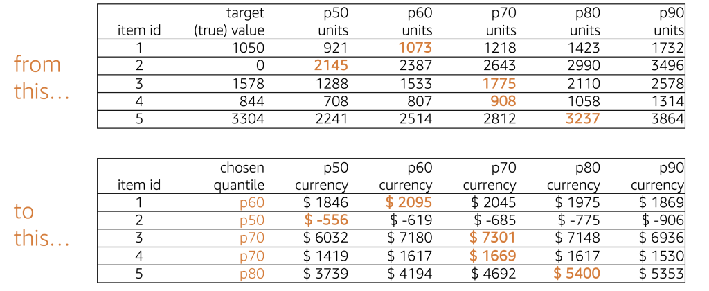
The following table demonstrates how the quantile points were self-selected from among the available forecast points in known historical periods. Consider the example of item 3, which had a true demand of 1,578 units in prior periods. A p50 estimate of 1,288 units would have undersupplied, whereas a p90 value of 2,578 units would have produced a surplus. Among the observed quantiles, the p70 value produces a maximum profit of $7,301. Knowing this, you can see how a p50 selection would result in a near $1,300 penalty, compared to the p70 value. This is only one example, but each item in the table has a unique story to tell.

Solution overview

The following diagram illustrates a proposed workflow. First, Amazon SageMaker Data Wrangler consumes backtest predictions produced by a time series forecaster. Next, backtest predictions and known actuals are joined with financial metadata on an item basis. At this point, using backtest predictions, a SageMaker Data Wrangler transform computes the unit cost for under and over forecasting per item.

SageMaker Data Wrangler translates the unit forecast into a financial context and automatically selects the item-specific quantile that provides the highest amount of profit among quantiles examined. The output is a tabular set of data, stored on Amazon S3, and is conceptually similar to the table in the previous section.

Finally, a time series forecaster is used to produce future-dated forecasts for future periods. Here, you may also choose to drive inference operations, or act on inference data, according to which quantile was chosen. This may allow you to reduce computational costs while also removing the burden of manual review of every single item. Experts in your company can have more time to focus on high-value items while thousands of items in your catalog can have automatic adjustments applied. As a point of consideration, the future has some degree of uncertainty. However, all other things being equal, a mixed selection of quantiles should optimize outcomes in an overall set of time series. Here at AWS, we advise you to use two holdback prediction cycles to quantify the degree of improvements found with mixed quantile selection.

Solution guidance to accelerate your implementation

If you wish to recreate the quantile selection solution discussed in this post and adapt it to your own dataset, we provide a synthetic sample set of data and a sample SageMaker Data Wrangler flow file to get you started on GitHub. The entire hands-on experience should take you less than an hour to complete.

We provide this post and sample solution guidance to help accelerate your time to market. The primary enabler for recommending specific quantiles is SageMaker Data Wrangler, a purpose-built AWS service meant to reduce the time it takes to prepare data for ML use cases. SageMaker Data Wrangler provides a visual interface to design data transformations, analyze data, and perform feature engineering.

If you are new to SageMaker Data Wrangler, refer to Get Started with Data Wrangler to understand how to launch the service through Amazon SageMaker Studio. Independently, we have more than 150 blog posts that help discover diverse sample data transformations addressed by the service.

Conclusion

In this post, we discussed how quantile regression enables multiple business decision points in time series forecasting. We also discussed the imbalanced cost penalties associated with over and under forecasting—often the penalty of undersupply is several multiples of the oversupply penalty, not to mention undersupply can cause the loss of goodwill with customers.

The post discussed how organizations can evaluate multiple quantile prediction points with a consideration for the over and undersupply costs of each item to automatically select the quantile likely to provide the most profit in future periods. When necessary, you can override the selection when business rules desire a fixed quantile over a dynamic one.

The process is designed to help meet business and financial goals while removing the friction of having to manually apply judgment calls to each item forecasted. SageMaker Data Wrangler helps the process run on an ongoing basis because quantile selection must be dynamic with changing real-world data.

It should be noted that quantile selection is not a one-time event. The process should be evaluated during each forecasting cycle as well, to account for changes including increased cost of goods, inflation, seasonal adjustments, new product introduction, shifting consumer demands, and more. The proposed optimization process is positioned after the time series model generation, referred to as the model training step. Quantile selections are made and used with the future forecast generation step, sometimes called the inference step.

If you have any questions about this post or would like a deeper dive into your unique organizational needs, please reach out to your AWS account team, your AWS Solutions Architect, or open a new case in our support center.

References

• DeYong, G. D. (2020). The price-setting newsvendor: review and extensions. International Journal of Production Research, 58(6), 1776–1804.
• Liu, C., Letchford, A. N., & Svetunkov, I. (2022). Newsvendor problems: An integrated method for estimation and optimisation. European Journal of Operational Research, 300(2), 590–601.
• Punia, S., Singh, S. P., & Madaan, J. K. (2020). From predictive to prescriptive analytics: A data-driven multi-item newsvendor model. Decision Support Systems, 136.
• Trapero, J. R., Cardós, M., & Kourentzes, N. (2019). Quantile forecast optimal combination to enhance safety stock estimation. International Journal of Forecasting, 35(1), 239–250.
• Whitin, T. M. (1955). Inventory control and price theory. Management Sci. 2 61–68.

---

About the Author

Charles Laughlin is a Principal AI/ML Specialist Solution Architect and works in the Amazon SageMaker service team at AWS. He helps shape the service roadmap and collaborates daily with diverse AWS customers to help transform their businesses using cutting-edge AWS technologies and thought leadership. Charles holds a M.S. in Supply Chain Management and a Ph.D. in Data Science.

• SEO Powered Content & PR Distribution. Get Amplified Today.
• PlatoData.Network Vertical Generative Ai. Empower Yourself. Access Here.
• PlatoAiStream. Web3 Intelligence. Knowledge Amplified. Access Here.
• PlatoESG. Carbon, CleanTech, Energy, Environment, Solar, Waste Management. Access Here.
• PlatoHealth. Biotech and Clinical Trials Intelligence. Access Here.
• Source: https://aws.amazon.com/blogs/machine-learning/beyond-forecasting-the-delicate-balance-of-serving-customers-and-growing-your-business/