Customer segmentation is the technique of diving customers into groups based on their purchase patterns to identify who are the most profitable groups. In segmenting customers, various criteria can also be used depending on the market such as geographic, demographic characteristics or behavior bases. This technique assumes that groups with different features require different approaches to marketing and wants to figure out the groups who can boost their profitability the most.
Today, we are going to discuss how to do customer segmentation analysis with the online retail dataset from UCI ML repo. This analysis will be focused on two steps getting the RFM values and making clusters with K-means algorithms. The dataset and the full code is also available on my Github. The original resource of this note is from the course “Customer Segmentation Analysis in Python.”
If this in-depth educational content on using AI in marketing is useful for you, you can subscribe to our Enterprise AI mailing list to be alerted when we release new material.
What is RFM?
RFM is an acronym of recency, frequency and monetary. Recency is about when was the last order of a customer. It means the number of days since a customer made the last purchase. If it’s a case for a website or an app, this could be interpreted as the last visit day or the last login time.
Frequency is about the number of purchase in a given period. It could be 3 months, 6 months or 1 year. So we can understand this value as for how often or how many a customer used the product of a company. The bigger the value is, the more engaged the customers are. Could we say them as our VIP? Not necessary. Cause we also have to think about how much they actually paid for each purchase, which means monetary value.
Monetary is the total amount of money a customer spent in that given period. Therefore big spenders will be differentiated with other customers such as MVP or VIP.
These three values are commonly used quantifiable factors in cohort analysis. Because of their simple and intuitive concept, they are popular among other customer segmentation methods.

Photo from CleverTap
Import the data
So we are going to apply RFM to our cohort analysis today. The dataset we are going to use is the transaction history data occurring from Jan 2010 to Sep 2011. As this is a tutorial guideline for cohort analysis, I’m going to use only the randomly selected fraction of the original dataset.
# Import data
online = pd.read_excel('Online Retail.xlsx') # drop the row missing customer ID
online = online[online.CustomerID.notnull()]
online = online.sample(frac = .3).reset_index(drop = True)
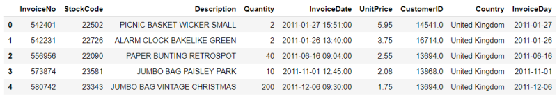
online.head()

Calculating RFM values
The first thing we’re going to count is the recency value, the number of days since the last order of a customer. From which column could we get that value? InvoiceData. With this column, we can get when was the first purchase and when was the last purchase of a customer. Let’s call the first one as CohortDay. As InvoiceDate also contains additional time data, we need to extract the year, month and day part. After that, we’ll get CohortDay which is the minimum of InvoiceDay.
 # extract year, month and day
online['InvoiceDay'] = online.InvoiceDate.apply(lambda x: dt.datetime(x.year, x.month, x.day)) online.head()
As we randomly chose the subset of the data, we also need to know the time period of our data. Like what you can see below, the final day of our dataset is December 9th, 2011. Therefore set December 10th as our pining date and count backward the number of days from the latest purchase for each customer. That will be the recency value.
 # print the time period
print('Min : {}, Max : {}'.format(min(online.InvoiceDay), max(online.InvoiceDay)))
![]()
![]()
 # pin the last date
pin_date = max(online.InvoiceDay) + dt.timedelta(1)
Before getting the recency, let’s count one more value in advance, the total amount of money each customer spent. This is for counting the monetary value. How can we get that? Easy! Multiplying the product price and the quantity of the order in each row.
 # Create total spend dataframe
online['TotalSum'] = online.Quantity * online.UnitPrice
online.head()

Now we are ready to get the three RFM values at once. I’ll group the data for each customer and aggregate it for each recency, frequency, and monetary value.
# calculate RFM values
rfm = online.groupby('CustomerID').agg({ 'InvoiceDate' : lambda x: (pin_date - x.max()).days, 'InvoiceNo' : 'count', 'TotalSum' : 'sum'}) # rename the columns
rfm.rename(columns = {'InvoiceDate' : 'Recency', 'InvoiceNo' : 'Frequency', 'TotalSum' : 'Monetary'}, inplace = True) rfm.head()

RFM quartiles
Now we’ll group the customers based on RFM values. Cause these are continuous values, we can also use the quantile values and divide them into 4 groups.
 # create labels and assign them to tree percentile groups
r_labels = range(4, 0, -1)
r_groups = pd.qcut(rfm.Recency, q = 4, labels = r_labels) f_labels = range(1, 5)
f_groups = pd.qcut(rfm.Frequency, q = 4, labels = f_labels) m_labels = range(1, 5)
m_groups = pd.qcut(rfm.Monetary, q = 4, labels = m_labels)
Please pay extra care for the r_labels. I gave the labels in descending order. Why is that? Because recency means how much time has elapsed since a customer’s last order. Therefore the smaller the value is, the more engaged a customer to that brand. Now let’s make a new column for indicating group labels.
 # make a new column for group labels
rfm['R'] = r_groups.values
rfm['F'] = f_groups.values
rfm['M'] = m_groups.values # sum up the three columns
rfm['RFM_Segment'] = rfm.apply(lambda x: str(x['R']) + str(x['F']) + str(x['M']), axis = 1)
rfm['RFM_Score'] = rfm[['R', 'F', 'M']].sum(axis = 1)
rfm.head()

I attached all three labels in one cell as RFM_Segment. In this way, we can easily check what level or segment a customer belongs to. RFM_Score is the total sum of the three values. It doesn’t necessarily have to be the sum so the mean value is also possible. Moreover, we can catch further patterns with the mean or count values of recency, frequency and monetary grouped by this score like below.
 # calculate averae values for each RFM
rfm_agg = rfm.groupby('RFM_Score').agg({ 'Recency' : 'mean', 'Frequency' : 'mean', 'Monetary' : ['mean', 'count']
}) rfm_agg.round(1).head()

RFM_Score will be the total score of a customer’s engagement or loyalty. Summing up the three values altogether, we can finally categorize customers into ‘Gold,’ ‘Silver,’ ‘Bronze,’ and ‘Green’.
 # assign labels from total score
score_labels = ['Green', 'Bronze', 'Silver', 'Gold']
score_groups = pd.qcut(rfm.RFM_Score, q = 4, labels = score_labels)
rfm['RFM_Level'] = score_groups.values rfm.head()

Great! We’re done with one cohort analysis with RFM values. We identified who is our golden goose and where we should take extra care. Now why don’t we try a different method for customer segmentation and compare the two results?
K-Means Clustering
K-Means clustering is one type of unsupervised learning algorithms, which makes groups based on the distance between the points. How? There are two concepts of distance in K-Means clustering. Within Cluster Sums of Squares (WSS) and Between Cluster Sums of Squares (BSS).

WSS means the sum of distances between the points and the corresponding centroids for each cluster and BSS means the sum of distances between the centroids and the total sample mean multiplied by the number of points within each cluster. So you can consider WSS as the measure of compactness and BSS as the measure of separation. For clustering to be successful, we need to get the lower WSS and the higher BSS.
By iterating and moving the cluster centroids, K-Means algorithm tries to get the optimized points of the centroid, which minimize the value of WSS and maximize the value of BSS. I won’t go more in-depth with the basic concept, but you can find a further explanation from video.

Photo from Wikipedia
Because K-means clustering uses the distance as the similarity factor, we need to scale the data. Suppose we have two different scales of features, say height and weight. Height is over 150cm and weight is below 100kg on average. So If we plot this data, the distance between the points will be highly dominated by height resulting in a biased analysis.
Therefore when it comes to K-means clustering, scaling and normalizing data is a critical step for preprocessing. If we check the distribution of RFM values, you can notice that they are right-skewed. It’s not a good state to use without standardization. Let’s transform the RFM values into log scaled first and then normalize them.
 # define function for the values below 0
def neg_to_zero(x):
if x <= 0:
return 1
else:
return x # apply the function to Recency and MonetaryValue column
rfm['Recency'] = [neg_to_zero(x) for x in rfm.Recency]
rfm['Monetary'] = [neg_to_zero(x) for x in rfm.Monetary] # unskew the data
rfm_log = rfm[['Recency', 'Frequency', 'Monetary']].apply(np.log, axis = 1).round(3)
The values below or equal to zero go negative infinite when they are in log scale, I made a function to convert those values into 1 and applied it to Recency and Monetary column, using list comprehension like above. And then, a log transformation is applied for each RFM values. The next preprocessing step is scaling but it’s simpler than the previous step. Using StandardScaler(), we can get the standardized values like below.
 # scale the data
scaler = StandardScaler()
rfm_scaled = scaler.fit_transform(rfm_log) # transform into a dataframe
rfm_scaled = pd.DataFrame(rfm_scaled, index = rfm.index, columns = rfm_log.columns)

The plot on the left is the distributions of RFM before preprocessing, and the plot on the right is the distributions of RFM after normalization. By making them in the somewhat normal distribution, we can give hints to our model to grasp the trends between values easily and accurately. Now, we are done with preprocessing.
What is the next? The next step will be selecting the right number of clusters. We have to choose how many groups we’re going to make. If there is prior knowledge, we can just give the number right ahead to the algorithm. But most of the case in unsupervised learning, there isn’t. So we need to choose the optimized number, and the Elbow method is one of the solutions where we can get the hints.
# the Elbow method
wcss = {}
for k in range(1, 11):
kmeans = KMeans(n_clusters= k, init= 'k-means++', max_iter= 300)
kmeans.fit(rfm_scaled)
wcss[k] = kmeans.inertia_ # plot the WCSS values
sns.pointplot(x = list(wcss.keys()), y = list(wcss.values()))
plt.xlabel('K Numbers')
plt.ylabel('WCSS')
plt.show()
Using for loop, I built the models for every number of clusters from 1 to 10. And then collect the WSS values for each model. Look at the plot below. As the number of clusters increases, the value of WSS decreases. There is no surprise cause the more clusters we make, the size of each cluster will decrease so the sum of the distances within each cluster will decrease. Then what is the optimal number?

The answer is at the ‘Elbow’ of this line. Somewhere WSS dramatically decrease but not too much K. My choice here is three. What do you say? Doesn’t it really look like an elbow of the line?
Now we chose the number of clusters, we can build a model and make actual clusters like below. We can also check the distance between each point and the centroids or the labels of the clusters. Let’s make a new column and assign the labels to each customer.
 # clustering
clus = KMeans(n_clusters= 3, init= 'k-means++', max_iter= 300)
clus.fit(rfm_scaled) # Assign the clusters to datamart
rfm['K_Cluster'] = clus.labels_
rfm.head()

Now we made two kinds of segmentation, RFM quantile groups and K-Means groups. Let’s make visualization and compare the two methods.
Snake plot and heatmap
I’m going to make two kinds of plot, a line plot and a heat map. We can easily compare the differences of RFM values with these two plots. Firstly, I’ll make columns to assign the two clustering labels. And then reshape the data frame by melting the RFM values into one column.
# assign cluster column
rfm_scaled['K_Cluster'] = clus.labels_
rfm_scaled['RFM_Level'] = rfm.RFM_Level
rfm_scaled.reset_index(inplace = True) # melt the dataframe
rfm_melted = pd.melt(frame= rfm_scaled, id_vars= ['CustomerID', 'RFM_Level', 'K_Cluster'], var_name = 'Metrics', value_name = 'Value')
rfm_melted.head()

This will make recency, frequency and monetary categories as observations, which allows us to plot the values in one plot. Put Metrics at x-axis and Value at y-axis and group the values by RFM_Level. Repeat the same code which groups the values by K_Cluster this time. The outcome would be like below.
# a snake plot with RFM
sns.lineplot(x = 'Metrics', y = 'Value', hue = 'RFM_Level', data = rfm_melted)
plt.title('Snake Plot of RFM')
plt.legend(loc = 'upper right') # a snake plot with K-Means
sns.lineplot(x = 'Metrics', y = 'Value', hue = 'K_Cluster', data = rfm_melted)
plt.title('Snake Plot of RFM')
plt.legend(loc = 'upper right')

This kind of plots is called ‘Snake plot’ especially in marketing analysis. It seems Gold and Green groups on the left plot are similar with 1 and 2 clusters on the right plot. And the Bronze and Silver groups seem to be merged into group 0.
Let’s try again with a heat map. Heat maps are a graphical representation of data where larger values were colored in darker scales and smaller values in lighter scales. We can compare the variance between the groups quite intuitively by colors.
 # the mean value in total
total_avg = rfm.iloc[:, 0:3].mean()
total_avg # calculate the proportional gap with total mean
cluster_avg = rfm.groupby('RFM_Level').mean().iloc[:, 0:3]
prop_rfm = cluster_avg/total_avg - 1 # heatmap with RFM
sns.heatmap(prop_rfm, cmap= 'Oranges', fmt= '.2f', annot = True)
plt.title('Heatmap of RFM quantile')
plt.plot()
And then repeat the same code for K-clusters as we did before.
# calculate the proportional gap with total mean
cluster_avg_K = rfm.groupby('K_Cluster').mean().iloc[:, 0:3]
prop_rfm_K = cluster_avg_K/total_avg - 1 # heatmap with K-means
sns.heatmap(prop_rfm_K, cmap= 'Blues', fmt= '.2f', annot = True)
plt.title('Heatmap of K-Means')
plt.plot()

It could be seen unmatching, especially at the top of the plots. But It’s just because of the different order. The Green group on the left will correspond to group 2. If you see the values inside each box, you can see the difference between the groups become significant for Gold and 1 group. And it could be easily recognized by the darkness of the color.
Conclusion
We talked about how to get RFM values from customer purchase data, and we made two kinds of segmentation with RFM quantiles and K-Means clustering methods. With this result, we can now figure out who are our ‘golden’ customers, the most profitable groups. This also tells us on which customer to focus on and to whom give special offers or promotions for fostering loyalty among customers. We can select the best communication channel for each segment and improve new marketing strategies.
Resources
This article was originally published on Towards Data Science and re-published to TOPBOTS with permission from the author.
Enjoy this article? Sign up for more updates on using AI in marketing.
We’ll let you know when we release more technical education.