Rodents such as rats and mice are associated with a number of health risks and are known to spread more than 35 diseases. Identifying regions of high rodent activity can help local authorities and pest control organizations plan for interventions effectively and exterminate the rodents.

In this post, we show how to monitor and visualize a rodent population using Amazon SageMaker geospatial capabilities. We then visualize rodent infestation effects on vegetation and bodies of water. Finally, we correlate and visualize the number of monkey pox cases reported with rodent sightings in a region. Amazon SageMaker makes it easier for data scientists and machine learning (ML) engineers to build, train, and deploy models using geospatial data. The tool makes it easier to access geospatial data sources, run purpose-built processing operations, apply pre-trained ML models, and use built-in visualization tools faster and at scale.

Notebook

First, we use an Amazon SageMaker Studio notebook with a geospatial image by following the steps outlined in Getting Started with Amazon SageMaker geospatial capabilities.

Data access

The geospatial image comes preinstalled with SageMaker geospatial capabilities that make it easier to enrich data for geospatial analysis and ML. For our post, we use satellite images from Sentinel-2 and the rodent activity and monkeypox datasets from open-source NYC open data.

First, we use the rodent activity and extract the latitude and longitude of rodent sightings and inspections. Then we enrich this location information with human-readable street addresses. We create a vector enrichment job (VEJ) in the SageMaker Studio notebook to run a reverse geocoding operation so that you can convert geographic coordinates (latitude, longitude) to human-readable addresses, powered by Amazon Location Service. We create the VEJ as follows:

import boto3
import botocore
import sagemaker
import sagemaker_geospatial_map region = boto3.Session().region_name
session = botocore.session.get_session()
execution_role = sagemaker.get_execution_role() sg_client= session.create_client( service_name='sagemaker-geospatial', region_name=region
)
response = sg_client.start_vector_enrichment_job( ExecutionRoleArn=execution_role, InputConfig={ 'DataSourceConfig': { 'S3Data': { 'S3Uri': 's3://<bucket>/sample/rodent.csv' } }, 'DocumentType': 'CSV' }, JobConfig={ "ReverseGeocodingConfig": { "XAttributeName": "longitude", "YAttributeName": "latitude" } }, Name='vej-reversegeo',
) my_vej_arn = response['Arn']

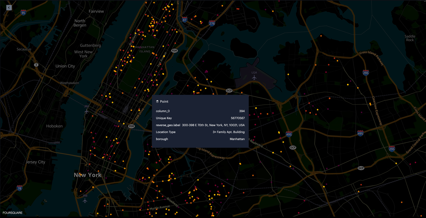
Visualize rodent activity in a region

Now we can use SageMaker geospatial capabilities to visualize rodent sightings. After the VEJ is complete, we export the output of the job to an Amazon S3 bucket.

sg_client.export_vector_enrichment_job( Arn=my_vej_arn, ExecutionRoleArn=execution_role, OutputConfig={ 'S3Data': { 'S3Uri': 's3://<bucket>/reversegeo/' } }
)

When the export is complete, you will see the output CSV file in your Amazon Simple Storage Service (Amazon S3) bucket, which consists of your input data (longitude and latitude coordinates) along with additional columns: address number, country, label, municipality, neighborhood, postal code, and region of that location appended at the end.

From the output file generated by VEJ, we can use SageMaker geospatial capabilities to overlay the output on a base map and provide layered visualization to make collaboration easier. SageMaker geospatial capabilities provide built-in visualization tooling powered by Foursquare Studio, which natively works from within a SageMaker notebook via the SageMaker geospatial Map SDK. Below, we can visualize the rodent sightings and also get the human readable addresses for each of the data points. The address information of each of the rodent sightings data points can be useful for rodent inspection and treatment purposes.

Analyze the effects of rodent infestation on vegetation and bodies of water

To analyze the effects of rodent infestation on vegetation and bodies of water, we need to classify each location as vegetation, water, and bare ground. Let’s look at how we can use these geospatial capabilities to perform this analysis.

The new geospatial capabilities in SageMaker offer easier access to geospatial data such as Sentinel-2 and Landsat 8. Built-in geospatial dataset access saves weeks of effort otherwise lost to collecting and processing data from various data providers and vendors. Also, these geospatial capabilities offer a pre-trained Land Use Land Cover (LULC) segmentation model to identify the physical material, such as vegetation, water, and bare ground, at the earth surface.

We use this LULC ML model to analyze the effects of rodent population on vegetation and bodies of water.

In the following code snippet, we first define the area of interest coordinates (aoi_coords) of New York City. Then we create an Earth Observation Job (EOJ) and select the LULC operation. SageMaker downloads and preprocesses the satellite image data for the EOJ. Next, SageMaker automatically runs model inference for the EOJ. The runtime of the EOJ will vary from several minutes to hours depending on the number of images processed. You can monitor the status of EOJs using the get_earth_observation_job function, and visualize the input and output of the EOJ in the map.

aoi_coords = [ [ [ -74.13513011934334, 40.87856296920188 ], [ -74.13513011934334, 40.565792636343616 ], [ -73.8247144462764, 40.565792636343616 ], [ -73.8247144462764, 40.87856296920188 ], [ -74.13513011934334, 40.87856296920188 ] ]
] eoj_input_config = { "RasterDataCollectionQuery": { "RasterDataCollectionArn": "arn:aws:sagemaker-geospatial:us-west-2:378778860802:raster-data-collection/public/nmqj48dcu3g7ayw8", "AreaOfInterest": { "AreaOfInterestGeometry": { "PolygonGeometry": { "Coordinates": aoi_coords } } }, "TimeRangeFilter": { "StartTime": "2023-01-01T00:00:00Z", "EndTime": "2023-02-28T23:59:59Z", }, "PropertyFilters": { "Properties": [{"Property": {"EoCloudCover": {"LowerBound": 0, "UpperBound": 2.0}}}], "LogicalOperator": "AND", }, }
}
eoj_config = { "LandCoverSegmentationConfig": {}
} response = geospatial_client.start_earth_observation_job( Name="eoj-rodent-infestation-lulc-example", InputConfig=eoj_input_config, JobConfig=eoj_config, ExecutionRoleArn=execution_role,
)
eoj_arn = response["Arn"]
eoj_arn Map = sagemaker_geospatial_map.create_map()
Map.set_sagemaker_geospatial_client(sg_client) Map.render() time_range_filter = { "start_date": "2023-01-01T00:00:00Z", "end_date": "2023-02-28T23:59:59Z",
} config = {"preset": "singleBand", "band_name": "mask"}
output_layer = Map.visualize_eoj_output( Arn=eoj_arn, config=config, time_range_filter=time_range_filter
)

To visualize the rodent population with respect to vegetation, we overlay the rodent population and sighting data on the land cover segmentation model predictions. This visualization can help us locate the population of rodents and analyze it on vegetation and bodies of water.

Visualize monkeypox cases and corelating with rodent data

To visualize the relation between the monkeypox cases and rodent sightings, we add the monkeypox dataset and the geoJSON file for New York City borough boundaries. See the following code:

nybb = pd.read_csv("./nybb.csv")
monkeypox = pd.read_csv("./monkeypox.csv")
dataset = Map.add_dataset({ "data": nybb
}, auto_create_layers=False)
dataset = Map.add_dataset({ "data": monkeypox
}, auto_create_layers=False)

Within a SageMaker Studio notebook, we can use the visualization tool powered by Foursquare to add layers in the map and add charts. Here, we added the monkeypox data as a chart to show the number of monkeypox cases for each of the boroughs. To see the correlation between monkeypox cases and rodent sightings, we have added the borough boundaries as a polygon layer and added the heatmap layer that represents rodent activity. The borough boundary layer is colored to match the monkeypox data chart. As we can see, the borough of Manhattan exhibits a high concentration of rodent sightings and records the highest number of monkeypox cases, followed by Brooklyn.

This is supported by a simple statistical analysis of calculating the correlation between the concentration of rodent sightings and monkeypox cases in each borough. The calculation produced an r value of 0.714, which implies a positive correlation.

r = np.corrcoef(borough_stats['Concentration (sightings per square km)'], borough_stats['Monkeypox Cases'])

Conclusion

In this post, we demonstrated how you can use SageMaker geospatial capabilities to get detailed addresses of rodent sightings and visualize the rodent effects on vegetation and bodies of water. This can help local authorities and pest control organizations plan for interventions effectively and exterminate rodents. We also correlated the rodent sightings to monkeypox cases in the area with the built-in visualization tool. By utilizing vector enrichment and EOJs along with the built-in visualization tools, SageMaker geospatial capabilities eliminate the challenges of handling large-scale geospatial datasets, model training, and inference, and provide the ability to rapidly explore predictions and geospatial data on an interactive map using 3D accelerated graphics and built-in visualization tools.

You can get started with SageMaker geospatial capabilities in two ways:

To learn more, visit Amazon SageMaker geospatial capabilities and Getting Started with Amazon SageMaker geospatial capabilitites. Also, visit our GitHub repo, which has several example notebooks on SageMaker geospatial capabilities.

About the authors

Bunny Kaushik is a Solutions Architect at AWS. He is passionate about building AI/ML solutions and helping customers innovate on the AWS platform. Outside of work, he enjoys hiking, rock climbing, and swimming.

Clarisse Vigal is a Sr. Technical Account Manager at AWS, focused on helping customers accelerate their cloud adoption journey. Outside of work, Clarisse enjoys traveling, hiking, and reading sci-fi thrillers.

Veda Raman is a Senior Specialist Solutions Architect for machine learning based in Maryland. Veda works with customers to help them architect efficient, secure and scalable machine learning applications. Veda is interested in helping customers leverage serverless technologies for Machine learning.

• SEO Powered Content & PR Distribution. Get Amplified Today.
• PlatoData.Network Vertical Generative Ai. Empower Yourself. Access Here.
• PlatoAiStream. Web3 Intelligence. Knowledge Amplified. Access Here.
• PlatoESG. Automotive / EVs, Carbon, CleanTech, Energy, Environment, Solar, Waste Management. Access Here.
• BlockOffsets. Modernizing Environmental Offset Ownership. Access Here.
• Source: https://aws.amazon.com/blogs/machine-learning/analyze-rodent-infestation-using-amazon-sagemaker-geospatial-capabilities/